Loopy Lattices

About a decade ago, Marko Rodrigez wrote a blog post on Loopy Lattices (see https://dzone.com/articles/big-data-graphs-loopy-lattices). It became infamous amongst graph database practitioners as it taught them a very important lesson: Never give in to the temptation to ask for all potential paths between two nodes. Never give in, never, never, never, never – in graphs great or small, large or petty, never give in to the temptation to ask for all paths, except to intentionally crash the server.
Let me explain. No, there is too much. Let me sum up (opens in a new tab): Imagine you take a graph, stretch it out and iron it, and when you do it turns out to look like a grid. This is a lattice (opens in a new tab).
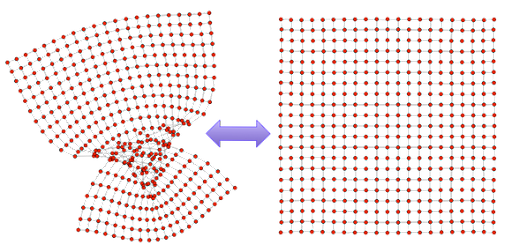
The grid-like graph above has 21 nodes across and 21 nodes down. There are 20 edges across and 20 down as well. This 20x20 lattice has a total of 441 nodes and 840 edges. By almost all measures, it is a tiny graph. Let’s imagine for a second this grid represents (opens in a new tab) roads and intersections. Think about getting around in Manhattan or Chicago, in Beijing or Kyoto. What if we were driving from the top-left node and needed to get to the bottom-right node? If you’ve seen gas prices lately, you probably understand the general importance of finding the shortest paths. Let’s see what happens when we ask just for the count of all the possible shortest paths from those two nodes. Maybe let’s start small with a 2x2 lattice.
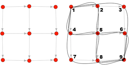
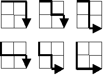
We need to get from Node 1 to Node 9. If you do this by hand, you will see a total of six possible shortest paths. All of the paths are four hops. The length is the width of the lattice plus the height of the lattice. Project Euler has an easy to follow picture for this problem (opens in a new tab):
Let’s keep going and try bigger graphs:

A 3x3 lattice has 20 shortest paths from the top-left node to the bottom-right node. There are 70 in a 4x4 lattice and 924 in a 6x6 lattice. At this level, it is too much to try to do this by hand. It quickly becomes too much for a traditional graph database. In the follow up post (opens in a new tab), Marko tells us that it took 10 minutes to calculate the answer up to 28 hops, 2.3 hours for 29 hops and almost 10 hours for 30 hops. He concluded that “the number of 40-length paths could not be reasonably calculated with titan/gremlin”.
Instead he turns from graph databases to the graph processing engine “Faunus” running on a hadoop cluster. It stores the count of the number of neighbors for each node and is able to brute force the answer much faster without as much traversing. Faunus is able to compute the total number of unique 40-length paths in the lattice in 10.53 minutes – 137,846,528,820. That is 137 billion paths in 10 minutes, almost 11… keep that in the back of your head.
Can we do better in Rel, RelationalAI’s declarative modeling language? Of course we can.
We get the correct answer: 137,846,528,820.
In how long? 0.41 seconds.
Do you want to know how? I’ll show you. Let’s start by building our graph. First, let’s define the size of our lattice and create the nodes:
Now we have 441 nodes, numbered 1 to 441. Let’s create the edges between them. Every node connects to the one to the right of it, except for those along the right side:
// means we have a 20x20 lattice. This is the
// number of edges per side.
def lattice_size = 20

// The number of nodes wide times the number of nodes high
// is equal to (20 + 1) * (20 + 1) = 441. For a 20x20 lattice,
// we need to create 441 nodes in the graph.
def number_of_nodes = (lattice_size + 1) * (lattice_size + 1)

// let's go ahead and create 441 nodes from 1 to 441
// incrementing by 1.
def node = range[1, number_of_nodes, 1]
// The node to the right is itself + 1. Node 8 connects
// to Node 9 and so on as long as we are not on the right
// side wall, which we are if we have a remainder from
// modulo[node_number, lattice_size + 1].
// For example 9 % 21 = 9. We're good.
// But 42 % 21 = 0, which means we are at the wall
// and we don't want to connect to the right.
def edge(node_number, right_node) = node(node_number) and
right_node = node_number + 1 and
modulo[node_number, lattice_size + 1] > 0Every node connects to the one down from it, except those along the bottom:
// For example, Node 8 connects to (8 + 20 + 1) = Node 29.
// But Node 434 can't connect down since it would connect
// to a node greater than 441.

def edge(node_number, down_node) = node(node_number) and
  down_node = node_number + lattice_size + 1 and
  down_node <= number_of_nodes
Notice how we have “def edge = ” twice? The second time is not overwriting it, it is saying that this is also equal to edge.
Now we have our graph. But how can we tell Rel what we want to do? How do we tell it we want to count the number of unique paths from node 1 to node 441?
In Rel, one of the things you have to get used to is recursive queries, which have these multiple “def statements”. Once you are able to think recursively, many problems become a lot easier. We start with the “base” case, which is usually the least exciting. Node 1 has a single path to itself of zero length:
def number_of_paths_of_length(node_number, path_length, path_count) =
	node_number=1, path_length=0, path_count=1
Now the exciting part… we define it again, this time saying that the number of paths of some length is also equal to the sum of the number of paths of (some length minus 1) of its neighbors.
def number_of_paths_of_length[node_number, path_length] =
    sum[other_node, paths_of_length : paths_of_length =
  	number_of_paths_of_length[other_node, path_length - 1]
  	and edge(other_node, node_number)]
It makes more sense with an example. How many paths of length 2 are there from Node 1 to Node 4 in this picture? The answer is the sum of the number of paths of length 1 from Node 1 to Node 2, plus the number of paths from Node 1 to Node 3. Okay, so how many of those are there?
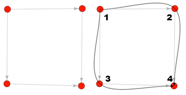
Well, we know there is one path of length 0 from Node 1 to itself. We also know an edge exists between Node 1 to Node 2 and another from Node 1 to Node 3, so if take the sum of these two formulas:
number_of_paths_of_length[node_one, path_length - 1] and
  edge(node_1, node_2)]

number_of_paths_of_length[node_one, path_length - 1] and
  edge(node_1, node_3)]
We get 1 + 1, which is our answer: 2 paths.
Let’s see it on a 2x2 lattice. From Node 1, there are three paths of length 3 to Node 6 and three paths of length 3 to Node 8. If we add them up, we get six, which is the number of paths of length 4 from Node 1 to Node 9.
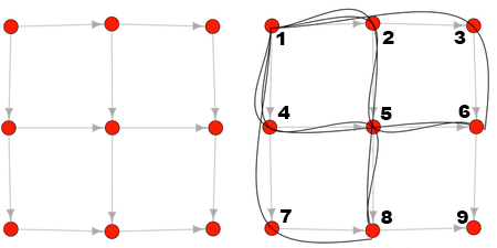
But wait, how do we know there are three paths of length 3 to Node 6? Well, there is just one path from Node 1 to Node 3 of length 2, from Node 1 to Node 2 to Node 3… and there are two paths of length 2 from Node 1 to Node 5. One goes by Node 2 and the other by Node 4.
How do we know Node 3 only has one path? Well, because it only connects to Node 2 which has only one path. How do we know Node 2 only has one path of length 1? Because it only connects to Node 1 and we already know that Node 1 has just one path to itself. So then how do we know Node 5 has two paths? It connects to Node 2, which we already established has one path from Node 1, and Node 4 only has one way to get to Node 1 which we already know is one. If we add them up, we get two paths.
If we keep going all the way to 20x20 and output our results:
def output = number_of_paths_of_length[number_of_nodes, 2 * lattice_size]What do we get?
// read query

def lattice_size = 20
def number_of_nodes = (lattice_size + 1) * (lattice_size + 1)
def node = range[1, number_of_nodes, 1]

def edge(node_number, right_node) = node(node_number) and right_node =
       node_number + 1 and modulo[node_number, lattice_size + 1] > 0

def edge(node_number, down_node) = node(node_number) and down_node =
       node_number + lattice_size + 1 and down_node <= number_of_nodes

def number_of_paths_of_length(node_number, path_length, path_count) =
       node_number=1, path_length=0, path_count=1

def number_of_paths_of_length[node_number, path_length] =
      sum[other_node, paths_of_length : paths_of_length =
         number_of_paths_of_length[other_node, path_length - 1] and edge(other_node, node_number)]

def output = number_of_paths_of_length[number_of_nodes, 2 * lattice_size]
The correct answer: 137,846,528,820 (on the bottom left) in 0.41 seconds (on the bottom right). It took a fraction of a second to calculate the 137 billion shortest paths from the top-left node to the bottom-right node in our lattice. That time blows 10 minutes out of the water. It is… I don’t even know how many orders of magnitude faster. So how did we do it? How were we able to compute the right answer so fast? To answer this question, we will talk about the semantic optimizer next time. Subscribe to our newsletter to be notified!
Do you want learn more about RelationalAI? Watch this video (opens in a new tab) from Martin Bravenboer (opens in a new tab). You can also take a look at all the code mentioned above at this link (opens in a new tab).
Related Posts

(RAI)volutionizing Master Data
Most master data projects fail because we've relied on monolithic MDM platforms, and therefore centralized, highly federated approaches to creating master data. The MDM concept is strong. The benefits and uses of master data can provide value to those corporations who successfully implement it. However, we need to fundamentally change our approach to implementation.

Trends in Machine Learning: ICLR 2022
This was the 10th ICLR conference, marking the golden decade of deep learning and AI. Despite early predictions that the deep learning hype would be ephemeral, we are happy to see the field still growing while delivering maturity in algorithms and architectures. ICLR 2022 was full of exciting papers. Here at RelationalAI we spent ~100 hours going through the content as we believe it will drive the commercialization of AI in the following years. Here we present what we found to be the most noteworthy ideas.